Table of Contents
Neural networks are trying to imitate abilities that the human (and animal) brain has, and the computers don’t. The first of those abilities is adaptability.
While a modern computer can outperform the human brain in any aspect. It is still a static device and that’s why it cannot use all its potential.
The artificial neural networks are trying to introduce brain functionalities to a computer by copying the behavior of the nervous systems.
But we can imagine Neural Network as a mathematical function that maps a given input set to the desired output set.
Neural Networks consist of the following components.
The diagram below shows the architecture of a 2-layer Neural Network. (Note that the input layer is typically excluded when counting the number of layers in a Neural Network).
Biases are not shown, but basically, they represent additional neurons (nodes) in the input and in the hidden layer(s), having a fixed value, for example, 1.
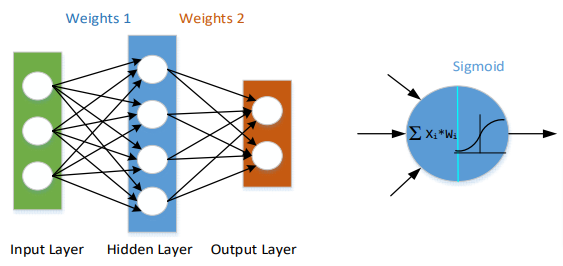
On the right-hand side of the diagram, you can see one such node in the hidden layer. At first, it sums up all the input signals, each affected by its weight coefficient. Then the sum is sent to the output, but at first, goes through a limiter.
The most popular limiter is implemented by the Sigmoid function S(x), as it can be relatively simply differentiated:
S(x) = 1 / (1 + e-x)
Similar nodes are used in the output layer, just their input signals are coming from the nodes of the hidden layer.
The right values for the weight coefficients determines the strength of the predictions, i.e. precision with which the input set will be transformed into the output set.
The process of fine-tuning the weights from the input data and hidden nodes is known as training the Neural Network. Each iteration of the training process consists of the following steps:
The output ŷ of a simple 2-layer Neural Network is calculated as:
ŷ = ϐ(W2ϐ(W1x + b1) + b2)
The predicted output will naturally differ from the desired output, at least at the beginning of the training process.
How much it differs will tell us the Loss Function. There are many available loss functions, but a simple, sum-of-squares error is a good loss function.
Sum-of-squares error = ∑(n, i=1) (𝑦 − ŷ)^2
Our goal in training is to find the best set of weights and biases that minimize the loss function.
Mathematically speaking we need to find a loss function extreme (minimum in our case).
The first derivation (its sign) will help us to find the direction, in which we need to modify the weights, and when the first derivation reaches zero, we should be in a (local) minimum of the function.
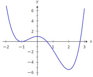
For example, the function below has two (local) minimums, one at x=-1 and the second one at x=2. If the function doesn’t have any other, more significant minimum, the second one is actually the global minimum.
And this is our goal, to find such weight coefficient values, which would yield the minimum in the loss function.
Of course, our loss function doesn’t depend on just one variable (x), but it is a multidimensional function. For more information about the Neural Network training look at the following, very nice explanation:
Let’s find the first derivation of the Sum-of-squares error function, ∂Loss(y,ŷ)/∂W.
Unfortunately, our loss function does not depend directly on the weight coefficients, so we need to apply the following chain rule in its derivation:
(∂ Loss(y,ŷ))/∂W = (∂ Loss(y,ŷ))/∂ŷ * ∂ŷ/∂z * ∂z/∂W
where z = ϐ(Wx + b)
Where the first partial derivation yields 2(y –)
the second partial derivation yields ϐ’
and the last partial derivation is just x
So, at the end we will get:
∂Loss(y,ŷ)/∂W = 2(y –) * ϐ’*x
and this is what we will have to implement as the backpropagation process. The advantage of the Sigmoid function is a simple implementation of its derivative:
ϐ’(u) = ϐ(u)(1 - ϐ(u)
The formula above describes how to proceed – backpropagate from the output of the neural network to the hidden layer, which stays in front of the output layer, and which is connected with the output layer via the W2 weights.
The same process has to be applied again going from the hidden layer to the input layer, which is connected with the hidden layer via the W1 weights.
The first chain member in the loss function derivation at the hidden layer, ∂Loss(h,ĥ)/∂ĥ, will have to be calculated differently, as we don’t explicitly know desired values of the hidden layer,h. We will need to calculate them from the output values.
Now we know everything is needed to implement such a simple Neural Network. We can start writing our program.
If you are new to the Python, check the complete Python tutorial.
For all the matrix operations we will use the NumPy library. This has to be imported at the very beginning of the source file.
import numpy as np
Let’s start with the Sigmoid function and its derivative definition:
def sigmoid(x):
     return 1.0/(1 + np.exp(-x))

def sigmoid_der(x):
     return x * (1.0 - x)
Notice how simply is the derivative of the Sigmoid function defined. Well, it could be done this way only because the x values have already passed through the Sigmoid function.
Now we are ready to define the NeuralNetwork class. Let’s call it NeuralNetwork1 as it will have just one hidden layer:
class NeuralNetwork1:

  def __init__(self, x, y, hln):
    np.random.seed(1)
    self.wih   = np.random.rand(x.shape[1], hln)
    #Input - Hidden Layer weights
    self.who   = np.random.rand(hln, y.shape[1])
    #Hidden -Output Layer weights
    self.inp   = x
    self.y     = y
    self.out   = np.zeros(self.y.shape)

  def feedforward(self):
    self.hid = sigmoid(np.dot(self.inp, self.wih))
    #Hidden Layer values
    self.out = sigmoid(np.dot(self.hid, self.who))
    #Output Layer values

  def backpropagation(self):
    # Start with the backpropagation from output to hidden layer
    out_err = 2*(self.y- self.out) # ∂Loss(y,ŷ)/∂y
    out_delta = out_err * sigmoid_der(self.out) # ∂Loss(y,ŷ)/∂y * ϐ’
    # This has to be calculated before who correction
    hid_err = np.dot(out_delta, self.who.T) # ∂Loss(h,ĥ)/∂ĥ
    # only now correct who weights
    self.who += np.dot(self.hid.T, out_delta) # W2 += ΔW2

    # Continue with the backpropagation from hidden to input layer
    hid_delta = hid_err * sigmoid_der(self.hid) # ∂Loss(h,ĥ)/∂ĥ * ϐ’
    # now correct wihweights
    self.wih += np.dot(self.inp.T, hid_delta) # W1 += ΔW1

  def__call__(self, Mi):
    hid = sigmoid(np.dot(Mi, self.wih)) #Hidden Layer values
    out = sigmoid(np.dot(hid, self.who)) #Output Layer values
    return out
In the class above, we are defining everything for the description of a neural network with one hidden layer. At the initialization, two matrices of weights will be created and filled with the random numbers in the <0.0,.,1.0> interval. Their size has to match the number of input, hidden and output nodes. The input and the desired output matrices are saved as the local variables.
The feedforward()method calculates the values of the output matrix. This is done in two stages, at first, the hidden matrix is created with the values calculated as a dot product of the input and weight W1 matrices.
The backpropagation() method is responsible for the weights W1 and W2 correction in such a way that the overall error at the output is minimized.
This is done again in two stages, the output stage has to be processed first. The first two statements represent the first two partial derivations (their product) of the derivation ∂Loss(y,ŷ)/∂W using the chain rule.
Before this product is multiplied with the third derivation member, input x, (in this case inputs are the hidden layer values), and the weights are corrected (the fourth statement), we can calculate the loss function at the hidden layer. As we do not have explicit values of the desired values at the hidden layer, we need to use the output layer error and backpropagate it to the hidden layer via (transposed) W2 weights.
What we get as hid_erractually corresponds to ∂Loss(h,ĥ)/∂ĥ, which is very convenient. Now we can finish the W2 weights correction and in the following two statements the values of the W1 weights as well.
The last method, __call__(Mi), can be used when you want to run your neural network for one particular input node combination, Mi.
And we have actually everything ready for the first experiment. Let’s write the following code in the Main section:
"""---------- Main function section ----------"""

if __name__ == "__main__":
  np.set_printoptions(suppress=True)
  #to suppress exp. format in print()
  np.set_printoptions(precision=3)
  #to set precision to 3 digits after decimal point

  """ These are all 4 combinations of two-bit input set """
  X1 = np.array([[0,0],[0,1],[1,0],[1,1]])

  """ This is corresponding output set combination
  to implement XOR function """
  y1 = np.array([[0],[1],[1],[0]])

  """ Here we will get result of the [X] -> [y] transformation
  where output becomes 1 when the input combination
  contains only one '1' value (i.e. XOR function)."""
  nn1 = NeuralNetwork1(X1, y1, 3)

  for i in range(10001):
  nn1.feedforward()
  if i == 10 or i == 1000 or i == 10000:
    print('Output set after %d steps:\n' %i)
    print(nn1.out)
    print("\n")
  nn1.backpropagation()
At first, we set few directives for the desirable printing of the data using the NumPy library. Then we defined the input matrix, which represents all combinations of two bits. And what we want from our neural network is a behavior of an XOR circuit, which will yield a value of 1 only when one of the two input bits have a value of 1. So, this is the y1matrix definition. Finally, we can instantiate the object nn1. We have defined there a hidden layer with 3 nodes.
In the following loop we run the nn1.feedforward() and nn1.backpropagation() methods (i.e. we train the nn1neural network) 10,000 times. To see how the training is progressing, at the 10-th, 1000-th, and at the last (10,000-th) cycle we print the output matrix values.
When we run the program above, we can clearly see, that even after 1000 cycles the neural network is completely “confused”, it shows all outputs indecisively as 0.5. Only after 10,000 training cycles, the output becomes clear, the “ones” values are almost 1.0, and “zeros” are almost 0.0. This was a pretty simple experiment, let’s try another, a more complex one.
Let the neural network recognize the digits between 0 and 9. This type of task is known as Pattern Recognition, and it is widely used in practice. In our experiment, we will create an input matrix as a set of 10 arrays each 99 bits long. Each array will represent a combination of “1” and “0” as they could be scanned by a sensor with 9 x 11 pixels, on which are images of those digits projected. For better visualization, we can write those arrays as matrices. To make the neural network more “robust”, let’s train it on two different patterns of each digit. If you look closely, you will recognize there each digit in two sizes, the first one contains a larger, while the second one contains a smaller version of the same digit:
X2 = np.array(
[[0,0,0,0,0,0,0,0,0,
 0,0,0,1,1,1,0,0,0,
 0,0,1,0,0,0,1,0,0, # 0
 0,1,0,0,0,0,0,1,0,
 0,1,0,0,0,0,0,1,0,
 0,1,0,0,0,0,0,1,0,
 0,1,0,0,0,0,0,1,0,
 0,1,0,0,0,0,0,1,0,
 0,0,1,0,0,0,1,0,0,
 0,0,0,1,1,1,0,0,0,
 0,0,0,0,0,0,0,0,0],

 [0,0,0,0,0,0,0,0,0,
 0,0,0,0,0,0,0,0,0,
 0,0,0,1,1,1,0,0,0, # 0
 0,0,1,0,0,0,1,0,0,
 0,0,1,0,0,0,1,0,0,
 0,0,1,0,0,0,1,0,0,
 0,0,1,0,0,0,1,0,0,
 0,0,1,0,0,0,1,0,0,
 0,0,0,1,1,1,0,0,0,
 0,0,0,0,0,0,0,0,0,
 0,0,0,0,0,0,0,0,0],

 [0,0,0,0,0,0,0,0,0,
 0,0,0,0,0,0,0,0,0,
 0,0,0,0,1,0,0,0,0, # 1
 0,0,0,0,1,0,0,0,0,
 0,0,0,0,1,0,0,0,0,
 0,0,0,0,1,0,0,0,0,
 0,0,0,0,1,0,0,0,0,
 0,0,0,0,1,0,0,0,0,
 0,0,0,0,1,0,0,0,0,
 0,0,0,0,0,0,0,0,0,
 0,0,0,0,0,0,0,0,0],

 [0,0,0,0,0,0,0,0,0,
 0,0,0,0,1,0,0,0,0,
 0,0,0,0,1,0,0,0,0, # 1
 0,0,0,0,1,0,0,0,0,
 0,0,0,0,1,0,0,0,0,
 0,0,0,0,1,0,0,0,0,
 0,0,0,0,1,0,0,0,0,
 0,0,0,0,1,0,0,0,0,
 0,0,0,0,1,0,0,0,0,
 0,0,0,0,1,0,0,0,0,
 0,0,0,0,0,0,0,0,0],

 [0,0,0,0,0,0,0,0,0,
 0,0,0,0,0,0,0,0,0,
 0,0,0,1,1,1,0,0,0, # 2
 0,0,1,0,0,0,1,0,0,
 0,0,0,0,0,0,1,0,0,
 0,0,0,0,0,1,0,0,0,
 0,0,0,0,1,0,0,0,0,
 0,0,0,1,0,0,0,0,0,
 0,0,0,1,1,1,1,0,0,
 0,0,0,0,0,0,0,0,0,
 0,0,0,0,0,0,0,0,0],

 [0,0,0,0,0,0,0,0,0,
 0,0,0,1,1,1,0,0,0,
 0,0,1,0,0,0,1,0,0, # 2
 0,1,0,0,0,0,0,1,0,
 0,0,0,0,0,0,0,1,0,
 0,0,0,0,0,0,1,0,0,
 0,0,0,0,0,1,0,0,0,
 0,0,0,0,1,0,0,0,0,
 0,0,0,1,0,0,0,0,0,
 0,0,1,1,1,1,1,1,0,
 0,0,0,0,0,0,0,0,0],

 [0,0,0,0,0,0,0,0,0,
 0,0,0,0,0,0,0,0,0,
 0,0,0,1,1,1,0,0,0, # 3
 0,0,1,0,0,0,1,0,0,
 0,0,0,0,0,1,0,0,0,
 0,0,0,0,1,0,0,0,0,
 0,0,0,0,0,1,0,0,0,
 0,0,1,0,0,0,1,0,0,
 0,0,0,1,1,1,0,0,0,
 0,0,0,0,0,0,0,0,0,
 0,0,0,0,0,0,0,0,0],

 [0,0,0,0,0,0,0,0,0,
 0,0,0,1,1,1,0,0,0,
 0,0,1,0,0,0,1,0,0, # 3
 0,1,0,0,0,0,0,1,0,
 0,0,0,0,0,0,1,0,0,
 0,0,0,0,0,1,0,0,0,
 0,0,0,0,0,0,1,0,0,
 0,1,0,0,0,0,0,1,0,
 0,0,1,0,0,0,1,0,0,
 0,0,0,1,1,1,0,0,0,
 0,0,0,0,0,0,0,0,0],

 [0,0,0,0,0,0,0,0,0,
 0,0,0,0,0,0,0,0,0,
 0,0,0,1,0,0,0,0,0, # 4
 0,0,0,1,0,0,0,0,0,
 0,0,1,0,0,0,0,0,0,
 0,0,1,1,1,1,1,0,0,
 0,0,0,0,1,0,0,0,0,
 0,0,0,0,1,0,0,0,0,
 0,0,0,0,1,0,0,0,0,
 0,0,0,0,0,0,0,0,0,
 0,0,0,0,0,0,0,0,0],

 [0,0,0,0,0,0,0,0,0,
 0,0,0,1,0,0,0,0,0,
 0,0,1,0,0,0,0,0,0, # 4
 0,0,1,0,0,0,0,0,0,
 0,1,0,0,0,0,0,0,0,
 0,1,1,1,1,1,1,1,0,
 0,0,0,0,1,0,0,0,0,
 0,0,0,0,1,0,0,0,0,
 0,0,0,0,1,0,0,0,0,
 0,0,0,0,1,0,0,0,0,
 0,0,0,0,0,0,0,0,0],

 [0,0,0,0,0,0,0,0,0,
 0,0,0,0,0,0,0,0,0,
 0,1,1,1,1,1,0,0,0, # 5
 0,1,0,0,0,0,0,0,0,
 0,1,0,0,0,0,0,0,0,
 0,1,1,1,1,0,0,0,0,
 0,0,0,0,0,1,0,0,0,
 0,1,0,0,0,1,0,0,0,
 0,0,1,1,1,0,0,0,0,
 0,0,0,0,0,0,0,0,0,
 0,0,0,0,0,0,0,0,0],

 [0,0,0,0,0,0,0,0,0,
 1,1,1,1,1,1,1,0,0,
 1,0,0,0,0,0,0,0,0, # 5
 1,0,0,0,0,0,0,0,0,
 1,0,0,0,0,0,0,0,0,
 1,1,1,1,1,1,0,0,0,
 0,0,0,0,0,0,1,0,0,
 0,0,0,0,0,0,1,0,0,
 1,0,0,0,0,1,0,0,0,
 0,1,1,1,1,1,0,0,0,
 0,0,0,0,0,0,0,0,0],

 [0,0,0,0,0,0,0,0,0,
 0,0,0,0,0,0,0,0,0,
 0,0,0,1,1,1,0,0,0, # 6
 0,0,1,0,0,0,1,0,0,
 0,0,1,0,0,0,0,0,0,
 0,0,1,1,1,0,0,0,0,
 0,0,1,0,0,1,0,0,0,
 0,0,1,0,0,0,1,0,0,
 0,0,0,1,1,1,0,0,0,
 0,0,0,0,0,0,0,0,0,
 0,0,0,0,0,0,0,0,0],

 [0,0,0,0,0,0,0,0,0,
 0,0,0,1,1,1,0,0,0,
 0,0,1,0,0,0,1,0,0, # 6
 0,1,0,0,0,0,0,1,0,
 0,1,0,0,0,0,0,0,0,
 0,1,0,1,1,1,0,0,0,
 0,1,0,0,0,0,1,0,0,
 0,1,0,0,0,0,0,1,0,
 0,0,1,0,0,0,1,0,0,
 0,0,0,1,1,1,0,0,0,
 0,0,0,0,0,0,0,0,0],

 [0,0,0,0,0,0,0,0,0,
 0,0,0,0,0,0,0,0,0,
 0,0,1,1,1,1,0,0,0, # 7
 0,0,0,0,0,1,0,0,0,
 0,0,0,0,0,0,0,0,0,
 0,0,0,0,1,0,0,0,0,
 0,0,0,0,1,0,0,0,0,
 0,0,0,1,0,0,0,0,0,
 0,0,0,1,0,0,0,0,0,
 0,0,0,0,0,0,0,0,0,
 0,0,0,0,0,0,0,0,0],

 [0,0,0,0,0,0,0,0,0,
 0,1,1,1,1,1,1,1,0,
 0,0,0,0,0,0,0,1,0, # 7
 0,0,0,0,0,0,1,0,0,
 0,0,0,0,0,1,0,0,0,
 0,0,0,0,1,0,0,0,0,
 0,0,0,0,1,0,0,0,0,
 0,0,0,1,0,0,0,0,0,
 0,0,0,1,0,0,0,0,0,
 0,0,0,1,0,0,0,0,0,
 0,0,0,0,0,0,0,0,0],

 [0,0,0,0,0,0,0,0,0,
 0,0,0,0,0,0,0,0,0,
 0,0,0,1,1,1,0,0,0, # 8
 0,0,1,0,0,0,1,0,0,
 0,0,1,0,0,0,1,0,0,
 0,0,0,1,1,1,0,0,0,
 0,0,1,0,0,0,1,0,0,
 0,0,1,0,0,0,1,0,0,
 0,0,0,1,1,1,0,0,0,
 0,0,0,0,0,0,0,0,0,
 0,0,0,0,0,0,0,0,0],

 [0,0,0,0,0,0,0,0,0,
 0,0,0,1,1,1,0,0,0,
 0,0,1,0,0,0,1,0,0, # 8
 0,1,0,0,0,0,0,1,0,
 0,0,1,0,0,0,1,0,0,
 0,0,0,1,1,1,0,0,0,
 0,0,1,0,0,0,1,0,0,
 0,1,0,0,0,0,0,1,0,
 0,0,1,0,0,0,1,0,0,
 0,0,0,1,1,1,0,0,0,
 0,0,0,0,0,0,0,0,0],

 [0,0,0,0,0,0,0,0,0,
 0,0,0,0,0,0,0,0,0,
 0,0,0,1,1,1,0,0,0, # 9
 0,0,1,0,0,0,1,0,0,
 0,0,1,0,0,0,1,0,0,
 0,0,0,1,1,1,1,0,0,
 0,0,0,0,0,0,1,0,0,
 0,0,1,0,0,0,1,0,0,
 0,0,0,1,1,1,0,0,0,
 0,0,0,0,0,0,0,0,0,
 0,0,0,0,0,0,0,0,0],

 [0,0,0,0,0,0,0,0,0,
 0,0,0,1,1,1,0,0,0,
 0,0,1,0,0,0,1,0,0, # 9
 0,1,0,0,0,0,0,1,0,
 0,0,1,0,0,0,1,1,0,
 0,0,0,1,1,1,0,1,0,
 0,0,0,0,0,0,0,1,0,
 0,1,0,0,0,0,0,1,0,
 0,0,1,0,0,0,1,0,0,
 0,0,0,1,1,1,0,0,0,
 0,0,0,0,0,0,0,0,0]])
It’s a lot of typing (at least it was for me), so you can just copy and paste the entire matrix into your source code.
Now, we need to define the output set. We have two options how to represent each digit. One option is to use binary coding, where with 4 bits we can encode each digit. Remember, each digit has to occur twice, exactly in the same order as are the corresponding input sets are coded:
y21 =np.array([[0,0,0,0],
             [0,0,0,0],
             [0,0,0,1],
             [0,0,0,1],
             [0,0,1,0],
             [0,0,1,0],
             [0,0,1,1],
             [0,0,1,1],
             [0,1,0,0],
             [0,1,0,0],
             [0,1,0,1],
             [0,1,0,1],
             [0,1,1,0],
             [0,1,1,0],
             [0,1,1,1],
             [0,1,1,1],
             [1,0,0,0],
             [1,0,0,0],
             [1,0,0,1],
             [1,0,0,1]])
This is the second option, to use “One in N” encoding:
y22= np.array([[0,0,0,0,0,0,0,0,0,1],
                    [0,0,0,0,0,0,0,0,0,1],
                    [0,0,0,0,0,0,0,0,1,0],
                    [0,0,0,0,0,0,0,0,1,0],
                    [0,0,0,0,0,0,0,1,0,0],
                    [0,0,0,0,0,0,0,1,0,0],
                    [0,0,0,0,0,0,1,0,0,0],
                    [0,0,0,0,0,0,1,0,0,0],
                    [0,0,0,0,0,1,0,0,0,0],
                    [0,0,0,0,0,1,0,0,0,0],
                    [0,0,0,0,1,0,0,0,0,0],
                    [0,0,0,0,1,0,0,0,0,0],
                    [0,0,0,1,0,0,0,0,0,0],
                    [0,0,0,1,0,0,0,0,0,0],
                    [0,0,1,0,0,0,0,0,0,0],
                    [0,0,1,0,0,0,0,0,0,0],
                    [0,1,0,0,0,0,0,0,0,0],
                    [0,1,0,0,0,0,0,0,0,0],
                    [1,0,0,0,0,0,0,0,0,0],
                    [1,0,0,0,0,0,0,0,0,0]])
And here is the second neural network object definition and the code for training:
    nn2 = NeuralNetwork1(X2, y21, 7)

    print('\nActual output matrix:\n')
    for i in range(10001):
        nn2.feedforward()
        if i == 100 or i == 1000 or i == 10000:
            print('Output after %d steps:\n' %i)
            print(nn2.out)
            print "\n"
        nn2.backpropagation()
When you run the program you will find out that the neural network has not been trained well. So, what went wrong?
Now replace the constant of 2 in the first statement in the backpropagation() method with a value of 1 (or delete this multiplication completely) and run the program again. Viola, it works!
What has changed? What we did is, that we made steps in finding the loss function minimum twice smaller. While this was not needed for the successful training of the XOR neural network, in this case, it is apparently needed.
And when you decide to represent the output values by the second way (y22), you will find out that even the step of 1.0* is too large to succeed. You will have to use the constant of 0.5 for successful training:
out_err = 0.5*(self.y- self.out)
This is nothing surprising in the finding extreme of a function. When you select large steps (Δx) you can easily miss the minimum, as you can end up bouncing well above it. So, why not to select a very tiny step increment.
Because you don’t know where are you on the function at the beginning, very small steps can lead you to the first (local) minimum, which can be far higher than the next one.
Imagine that you start looking for the minimum of the loss function (shown as the second picture in this article) at the x value of -2 and the steps, Δx, are something like 0.1. For sure this will get you to the minimum, but unfortunately, it will be the first minimum at x = -1. You will never learn that there is another, far lower minimum at x = 2.
If we selected larger steps, we might “jump” to the area around the second minimum, but then we might end-up bouncing around it and never reaching its bottom.
After the successful training we can run our neural network to provide a result for any combination of the input nodes, like for example this “distort” digit 3:
 # Test it to recognize number 3
     Xin = np.array(
         [0,0,0,0,0,0,0,0,0,
          0,0,0,0,0,0,0,0,0,
          0,0,0,1,1,1,0,0,0,  # 3
          0,0,1,0,0,0,1,0,0,
          0,0,0,0,0,1,0,0,0,
          0,0,0,0,1,0,0,0,0,
          0,0,0,0,0,1,0,0,0,
          0,0,0,0,0,0,1,0,0,
          0,0,1,0,0,0,0,1,0,
          0,0,0,1,1,1,1,0,0,
          0,0,0,0,0,0,0,0,0])

 Yout = nn2(Xin)
     print("\nResult for the selectedinput data set:")
     print Yout;
So, challenge # 1 for further neural network improvement might be finding the most appropriate steps in the loss function investigation. You might need to apply a variable step value, something which is known as step halving.
We can improve the speed of tuning by adding the bias values to the input and hidden nodes. To do so for the input layer is easy, let’s modify the input matrix, X1, as follows:
X1 = np.array([[1,0,0],[1,0,1],[1,1,0],[1,1,1]])
where we extended number of the columns by one, and as the first column value in each row we have placed a value of 1.
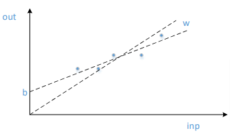
Is the bias important? Yes, it is as it can vastly improve convergence and the final neural network solution. What we are actually doing with the training, we are trying to optimize all the weights values, so they could make the optimal transformation of the input values to the output values. But adding the bias is like adding an offset to the linear function. It can make a significant difference.
Similarly, it would be desirable to add another node to the hidden layer, which as well will be set to 1. But let this be challenge # 2 because this is far complicated than as it was for the input layer.
There are other challenges, like extending the number of neural network hidden layers and finding out the optimal number of their nodes. Of course, the Neural Network is a huge scientific discipline, which, like all other scientific disciplines, requires dedicated investigations, studying, and experimentation. So, good luck to you if you want to proceed in this field.

Peter Galan is (now retired) control system designer with extensive experience in electronics, control systems and software design. He worked for many companies like ZTS, GE, Husky, Nortel, JDSU (in Canada) and previously at the Technical University in Kosice (today’s Slovakia). He holds a Ph.D. degree in Automated Control Systems and M.Eng degree in Applied Cybernetics (from Czech Technical University in Prague).
I made further experiments and found a significant improvement! Instead of the initial filling the wih and who matrices by the random numbers from the interval, try to fill them with the symmetrically spaced random numbers around 0, like the following
    self.wih   = np.random.rand(x.shape[1], hln) - 0.5
    #Input - Hidden Layer weights
    self.who   = np.random.rand(hln, y.shape[1]) - 0.5
    #Hidden -Output Layer weights