[Tutorial] Control Systems Simulation in Python | Example

Control systems belong among the essential engineering achievements.

We take them as something completely natural, but the control system designers have to struggle before they succeed in their job.

Yes, there are available many simulation systems, like Simulink (under Matlab), but if you need to implement (not just to design and tune) such a control system, using a suitable, general-purpose programming language, is more desirable.

If you are such a control system designer, you might find in this tutorial some interesting aspects, which can help you in your effort.

At the end of this tutorial you will be able to develop control systems simulation in Python

But for the refreshment, let’s start with the basic theory of control systems. 

1. Control Systems Introduction

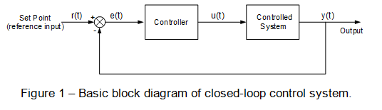
Figure 1 shows a basic block diagram of a generic, closed-loop control system. It consists of the Controlled System or Plant and the Controller. 

The purpose of the controller is to maintain the output variable at the level determined by the reference input.

This is accomplished by the comparison (subtraction) of the output variable, and the reference input.

The result is a regulation error, which is input information for the controller.

The controller calculates the actuating variable, which is the input to the controlled system. 

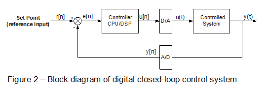
While the controlled systems are predominantly analog systems (i.e. they could be described by the continuous-time mathematical equations), today’s controllers are predominantly digital systems, so the block diagram of such a closed-loop control system can be represented rather by Figure 2.  Two new components are the D/A and A/D converters.

Only two signals,  and are of the continuous-time character. The remaining signals are all in the discrete form. 

So, the entire signal processing including the comparison of and can be accomplished by a suitable digital system (a microcontroller, for example). 

2. System Analysis

The first phase of a control system design is the controlled system (plant)analysis. You need to extract as much information about the controlled system as possible.

For the control purposes we are interested in the transfer function of the system, preferably in a well-known (s-domain) form:

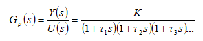
If you are designing the controlled system yourself, then you might be able to model (describe) it with a set of differential equations. It sounds easy, but even for the simplest controlled system, like a DC servo motor, it can take an enormous amount of time to finalize its mathematical description.

If you cannot mathematically describe your controlled system, you have to treat it as a “black box” and to find its transfer function in a different way. The best way is to apply a step function at the input to the system and to capture and plot its time response. What you will get will be very likely an “S” shaped curve as it is shown in Figure 3.

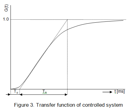
Now plot a tangent line going through the inflection point of the curve as it is shown in Figure 3. On the time (t) axis you should be able to mark two distinguished line segments, T_uand T_n.  From their ratio you will be able to determine not only the order of the transfer function, but in the case of the most common, second-order transfer function, you can find out both time constants.

In this tutorial we are not going any deeper into the controlled system analysis, please find other articles/tutorials, which are providing more information. One such article I wrote and published at ControlEng.

It might not be available there anymore, so if you are still interested in it, please let me know in the discussion at the end of this tutorial.  

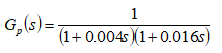
Anyway, you might find that your controlled system is equivalent to the second-order system with the following transfer function (where Gain is one for simplicity).

So, how Python can help with the simulation of your controlled system?

Well, at first we need to find the way how to describe such continuous-time systems with the discrete-time tools.

We shall start with a simpler, first-order system.

What is first-order system?

A first-order system can be described as a recursive filter or Infinite Impulse Response (IIR) filter.

The output of such a filter can be mathematically described as the sum of the following difference equation:

y[n] = a0x[n] + a1x[n-1] + a2x[n-2] + … + b1y[n-1] + b2y[n-2] + …

where

• y[n], y[n-1],… are the system (filter) outputs at the current timestamp, n, previous timestamp, n-1 etc., and
• x[n], x[n-1], … are theinput values to the system at the current timestamp, n, previous timestamp, n-1 etc.
• a₀, a₁,… b1, b₂,… are the weight coefficients forming the convolution kernel. They are usually referred to as the recursion coefficients.

We are going to look closely into a single pole (i.e. first-order) low-pass filter, as with this onewe will be able to simulate the transfer function of any controlled system.

Output of such a basic filter is:

y[n] = a0x[n] + b1y[n-1]

For the synthesis of control systems is useful to know the transfer function (i.e. y/x ratio), which in the case of this simple, first-order low-pass filter, is:

H[z] = a0 / (1 – b1z-1) 

Now we need to find the relation between those two, a₀ and b₁, coefficients, and the time constant of a corresponding single-pole filter.

In an RC (analog) filter the R*C product represents the time constant of a filter, i.e. the time (in seconds), which takes an RC filter output to rise to 63.2% of its input (step function) value, or decay to 36.8% of its original step function value (if such an RC filter is a high-pass filter).

This rise or decay follows a simple exponential function.

For a single-pole low-pass filter there is a simple rule for selection of those two coefficients:

a0= 1 - x

b1= x

And what is x?

It is a value between 0 and 1, and it actually represents the amount of decay (or rise) between two samples.

The higher number, the slower decay/rise.

In a discrete-time representation, we are rather interested in the representation of this decay/rise in terms of samples.

For example, we want to create a recursive filter with the “time constant” of 10 samples, which means that after exactly ten samples (steps or iterations) the filter output will decay/rise exactly by that 63.2 %.

Here is a simple formula, which expresses the decay coefficient, x, by a number of samples, d:

How to create simulation in Python?

To create simulation, you should have the basic Python programming skills.

Now we can write a code for a class representing such a recursive, low-pass filter:

class LowPassFilter: # H[z] = a0 / (1 - b1 * z ^ -1)
  # value of d means the number of samples, i.e. T(for 63.2 % rise)
  def __init__(self, d):
    if d > 0:
      e = -1.0 / d
      x = math.exp(e)
    else:
      x = 0
    self.b1 = x
    self.a0 = 1 - self.b1
    self.Ypr = 0

  def __call__(self, X):
    Y = self.a0 * X + self.b1 * self.Ypr
    self.Ypr = Y
    return Y

When we instantiate an object of the LowPassFilter class, we will prepare for it the a₀ and b₁ coefficients based on the desired number of samples, d, representing the “time constant” of the filter.

When we then call this object (as a function) with an argument representing the step function value, it will return the filter output after one iteration.

You can easily verify how your filter performs by adding the following code to your source file:

if __name__ == "__main__":
  Lpf = LowPassFilter(10)
    for i in range (1, 100):
      print 'step ' + str(i) + ' output: ' + str(Lpf(100)) 

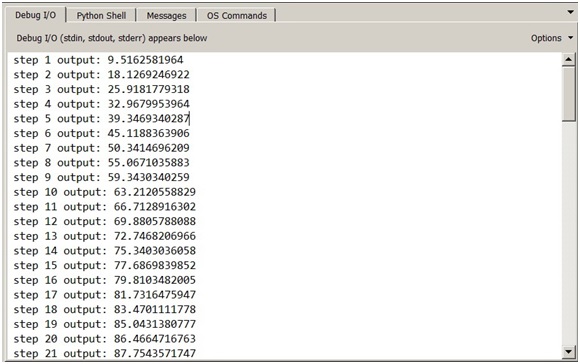
Below is the output of the program above. You can clearly see that the filter output after 10-th iteration is exactly 63.2 (actually, it is shown with a much higher precision) percent of the input value (100%).

Can we now simulate, for example, the above shown second-order transfer function?

Actually yes, we can. We just would need to “connect” two, first-order systems (low-pass filters) into a cascade, like:

if __name__ == "__main__":
  Lpf1 = LowPassFilter(4)
  Lpf2 = LowPassFilter(16)

  for i in range (1, 100):
    print 'step ' + str(i) + ' output: ' + str(Lpf2(Lpf1(100)))

where we replaced the original time constants of 4ms and 16ms by 4 and 16 samples/iteration steps resp.

This selection makes our “sampling” rate to be exactly one sample per 1ms.

It will work, just the sampling would be a little bit “rough”, as to have just 4 samples of the time constant is a little bit too few samples. Ten times higher sampling rate would be better. But then you wouldn’t want to print a thousand values in the output console and analyze them, you would prefer to see the output values in a graphical form.

With Python, even this is easily possible.

You would need to use some visual/graphical library, which would allow you to write such a program.

I personally like the VPython library, which however supports only Python 2 versions, so for Python 3 you need to use some other visual library.

Before we go any further, we should understand how many samples (iteration steps) we would need to take from the analyzed systems like is ours.

So, for such “exponentially” behaving systems, it takes around 5 times more time than is their time constant to exhibit “stabilized” output.

Our second-order system has a combined/total time constant of 20ms (4 + 16), so capturing a 100ms interval is what we need.

And taking 10 samples of the 1ms interval is reasonable as well. So, count on taking 1000 samples.

While we can simulate any second-order system by a cascade of two, first-order systems, it is not a very elegant way, as we can easily write a code of a second-order system – low-pass filter, as for example the following:

class SecondOrderSystem: 
  def __init__(self, d1, d2):
    if d1 > 0:
      e1 = -1.0 / d1
      x1 = math.exp(e1)
    else: x1 = 0
    if d2 > 0:
      e2 = -1.0 / d2
      x2 = math.exp(e2)
    else: x2 = 0
    a = 1.0 - x1    # b = x1
    c = 1.0 - x2    # d = x2
    self.ac = a * c
    self.bpd = x1 + x2
    self.bd = x1 * x2
    self.Yppr = 0
    self.Ypr = 0

  def __call__(self, X): 
    Y = self.ac * X + self.bpd * self.Ypr - self.bd * self.Yppr
    self.Yppr = self.Ypr
    self.Ypr = Y
    return Y

This class constructor gets two parameters, d₁ and d₂ when the object is instantiated, and inside the a₀ and b₁ coefficients of two such first-order systems are prepared and calculated, named as a  and b (i.e. x1) (first system) and c and d (i.e. x2) (second system).

Then their combined coefficients are created and calculated to implement the second-order transfer function:

H[z] = a0 / (1 – b1z-1) * c0 / (1 – d1z-1)= a0c0 / (1 – (b1+d1)z-1  + b1d1z-2  )

which is used to calculate the system output when you call the object as a function and provide the input value as an argument.

3. System Synthesis

The controlled process is usually a continuous process, so all the variables are continuous functions of time. 

On the other side, digital processor-based closed-loop controllers instead of using continuous-time signals (reference inputs, actual values, etc.) they process only digitized samples of those analog signals. Such systems are best described in the z-domain. 

However, the entire control system synthesis can be done in the s-domain, and switching to the z-domain can be done in the implementation phase.

From the control theory, you can remember that PID (proportional, integral, derivative) compensation is one of the most common forms of closed-loop control. 

Why PID controller is so popular? 

In most applications, the controlled process can be expressed by a first or a second-order transfer function.

And the PID controller can cancel, or at least significantly compensate exactly two poles of the transfer function.

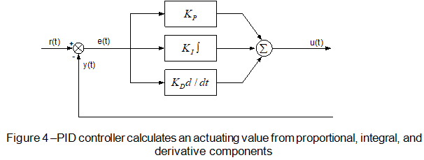
Figure 4 shows such a continuous-time (analogue) PID controller.

The controller calculates the regulation error, e(t), as a difference between the reference value or setpoint, r(t) , and the actual output value, y(t).

Then the proportional component of the controller multiplies this error signal by a proportional constant, Kp.

The integration component calculates an integral of e(t) and multiplies it by an integral constant, K1. The derivative member calculates a derivative of e(t) and multiplies it by a derivative constant, Kd.

The sum of these three components creates the actuating value, u(t) , which is applied to the controlled system.

This is the differential equation of the PID control block output as a function of the regulation error:

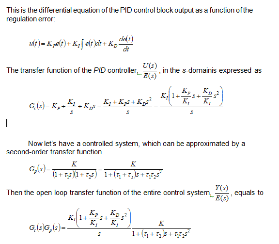
And here you can see why such a PID controller is so important.

You can optimally tune its parameters like the Kp/Ki ratio can match the value of T1+T2 sum and the Kd/Ki ratio can match the value T1*T2 of the product.

The open-loop transfer function will be reduced just to: (K1.K)/s as both poles of the transfer function have been “canceled”.

In such an optimally tuned control system the closed-loop transfer function becomes just a first-order low-pass (filter) system with the time constant, T1, equivalent to 1/Ki.

This is very good because we can achieve a much faster time response from the closed-loop control system (if you make K1 adequately large) than what is the response of the controlled system itself.

4. Control System Implementation

The analog PID controller can be easily modified to be implemented as a discrete-time control system, as it is not difficult to rewrite the differential equation of the PID controller into its difference form:

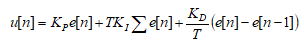
Where,

• u[n] is the actuating value at the present time n
• e[n] is the regulation error at the time n
• e[n-1] is the regulation error at the previous sample time, n-1. 
• T is the time period of the sampling.  The same time period, T, is used for the processing, i.e. for u[n] calculation.

For practical applications, certain modifications of this equation are needed. 

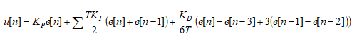
At first, the integral member will better use the trapezoidal approximation of integration instead of the rectangular one.

Then the derivative member tends to be noisy.

To reduce noise, we can use more than two (for example four) consecutive samples of the regulation error and put them through a tiny (4-tap) FIR filter.

Here is the modified PID formula:

The difference equation above can be easily implemented in Python, for example:

class PIDControlBlock:
  def __init__(self, Kp, Ki, Kd):
    self.Kp = Kp
    self.Ki = Ki
    self.Kd = Kd
    self.Epr = 0
    self.Eppr = 0
    self.Epppr = 0
    self.Sum = 0

  def __call__(self, E): 
    self.Sum += 0.5 * self.Ki * (E + self.Epr)      # where T ~1
    U = self.Kp * E + self.Sum + 0.1667 * self.Kd * (E - self.Epppr + 3.0 * (self.Epr - self.Eppr))
    self.Epppr = self.Eppr
    self.Eppr = self.Epr
    self.Epr = E
    return U

As we already have the controlled system (plant) class designed, we can put together those two and create the final, ClosedLoopSystem class:

class ClosedLoopSystem:
  def __init__(self, controller, plant) :
    self.P = plant
    self.C = controller
    elf.Ypr = 0

  def __call__(self, X):
    E = X - self.Ypr
    U = self.C(E)
    Y = self.P(U)
    self.Ypr = Y
    return Y

And here is the code, with which you can simulate the entire closed-loop control system.

The Plant object is represented as a second-order system with the time constants 250ms and 100ms (or iteration/sample numbers).

The Pid object is instantiated with the optimal, Kp, Ki, Kd, coefficients, and with the selected Ki value, it will make the closed-loop response 5-times faster than the combined time constant of the plant.  

if __name__ == "__main__":
  Plant = SecondOrderSystem(250, 100)     
  Pid = PIDControlBlock(5, 0.0143, 356.25
  Ctrl = ClosedLoopSystem(Pid, Plant)

  for i in range(1, 1001):
    print str(Ctrl(100))

However, the best way to simulate such processes is via plotting the diagrams.

Here you can see,

• the time (sample) response of the exact same controlled system (blue)
• an optimally tuned closed-loop control system (yellow)
• an overcompensated closed-loop system (red).

5. Conclusion

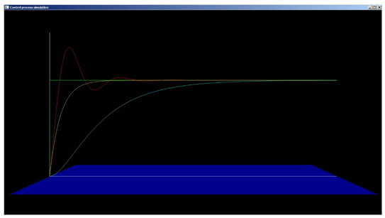
This tutorial shows how such complex systems like the control systems can be relatively very easily simulated in Python.

Especially for non-programmers, Python (which can be easily learned) can play an important role in the design of such engineering projects.

As a professional programmer, I write more complex applications usually in C#, but I am still using Python as a “scratchpad”, whenever I get some new ideas.

This was exactly the case with the subject of this tutorial.

Well, before that I implemented the same PID formula in many embedded projects, where of course neither Python nor C# could be used.

Everything had to be written in C and the most critical parts even in the assembly code.

Later, after creating this simulation program in Python I wrote an “extended” application in C#, which provides far more options, like you can tune the Kp, Ki, Kd, coefficients manually and see immediately their impact on the system behavior:

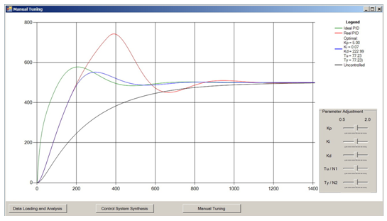
The same application could be written in Python, but for PC applications running under MS Windows C# is an obvious choice.

However, if you are a scientist or a professional other than a computer programmer, Python is the best language, which can help you in many of your endeavors.

This is all about control systems simulation in Python. If you have any questions, you can ask me in the comment section below.

Peter Galan

Peter Galan is (now retired) control system designer with extensive experience in electronics, control systems and software design. He worked for many companies like ZTS, GE, Husky, Nortel, JDSU (in Canada) and previously at the Technical University in Kosice (today’s Slovakia). He holds a Ph.D. degree in Automated Control Systems and M.Eng degree in Applied Cybernetics (from Czech Technical University in Prague).